CEDAR

Complex-systems Exploration and Design via Agent-Orchestrated Refinement

Agent-Orchestrated Tree Search for Goal-Directed Optimization of Complex Systems

Yingtao Tian / Sakana AI / [email protected] / @alanyttian
ALIFE 2026: The 2026 Conference on Artificial Life

goal = "grow population stably"▌

01 / The pitch

What if we could ask for a better world, in plain language?

World Dynamics (Forrester, 1971): a classic hand-designed model of population, resources, and pollution. Now just ask:

Balance population, resources, and environment by optimizing to (1) maximize population growth, (2) minimize the resource depletion rate, and (3) minimize the pollution accumulation rate. Seek the best trade-off where the population grows sustainably...

No equations to derive. No DYNAMO or STELLA to learn. No manual trial-and-error.
CEDAR takes this sentence and autonomously evolves the system: ~30 minutes, $10–$50 per run.

This talk: how LLM agents + tree search make that work, and what it offers artificial life.

        *       WORLD DYNAMICS W5

1       L       P.K = P.J + (DT)*(BR.JK - DR.JK)
1.1     N       P = PI
1.2     C       PI = 1.65E9

2       R       BR.KL = P.K * CLIP(BRN, BRN1, SWT1, TIME.K) * BRFM.K * BRMM.K * BRCM.K * BRPM.K
2.2     C       BRN = 0.04
2.3     C       BRN1 = 0.04
2.4     C       SWT1 = 1970

3       A       BRMM.K = TABHL(BRMMT, MSL.K, 0, 5, 1)
3.1     T       BRMMT = 1.2 / 1 / 0.85 / 0.75 / 0.7 / 0.7

4       A       MSL.K = ECIR.K / ECIRN
4.1     C       ECIRN = 1

5       A       ECIR.K = CIR.K * (1 - CIAF.K) * NREM.K / (1 - CIAFN)

6       A       NREM.K = TABLE(NREMT, NRFR.K, 0, 1, 0.25)
6.1     T       NREMT = 0 / 0.15 / 0.5 / 0.85 / 1

7       A       NRFR.K = NR.K / NRI

8       L       NR.K = NR.J + (DT)*(-NRUR.JK)
8.1     N       NR = NRI
8.2     C       NRI = 900E9

9       R       NRUR.KL = P.K * CLIP(NRUN, NRUN1, SWT2, TIME.K) * NRMM.K
9.1     C       NRUN = 1
9.2     C       NRUN1 = 1
9.3     C       SWT2 = 1970

        NOTE    EQUATION 42 CONNECTS HERE FROM EQ. 4 TO EQ. 9

10      R       DR.KL = P.K * CLIP(DRN, DRN1, SWT3, TIME.K) * DRMM.K * DRPM.K * DRFM.K * DRCM.K
10.2    C       DRN = 0.028
10.3    C       DRN1 = 0.028
10.4    C       SWT3 = 1970

11      A       DRMM.K = TABHL(DRMMT, MSL.K, 0, 5, 0.5)
11.1    T       DRMMT = 3 / 1.8 / 1 / 0.8 / 0.7 / 0.6 / 0.53 / 0.5 / 0.5 / 0.5 / 0.5

12      A       DRPM.K = TABLE(DRPMT, POLR.K, 0, 60, 10)
12.1    T       DRPMT = 0.92 / 1.3 / 2 / 3.2 / 4.8 / 6.8 / 9.2

13      A       DRFM.K = TABHL(DRFMT, FR.K, 0, 2, 0.25)
13.1    T       DRFMT = 30 / 3 / 2 / 1.4 / 1 / 0.7 / 0.6 / 0.5 / 0.5

14      A       DRCM.K = TABLE(DRCMT, CR.K, 0, 5, 1)
14.1    T       DRCMT = 0.9 / 1 / 1.2 / 1.5 / 1.9 / 3

15      A       CR.K = P.K / (LA * PDN)
15.1    C       LA = 135E6
15.2    C       PDN = 26.5

16      A       BRCM.K = TABLE(BRCMT, CR.K, 0, 5, 1)
16.1    T       BRCMT = 1.05 / 1 / 0.9 / 0.7 / 0.6 / 0.55

17      A       BRFM.K = TABHL(BRFMT, FR.K, 0, 4, 1)
17.1    T       BRFMT = 0 / 1 / 1.6 / 1.9 / 2

18      A       BRPM.K = TABLE(BRPMT, POLR.K, 0, 60, 10)
18.1    T       BRPMT = 1.02 / 0.9 / 0.7 / 0.4 / 0.25 / 0.15 / 0.1

19      A       FR.K = FPCI.K * FCM.K * FPM.K * CLIP(FC, FC1, SWT7, TIME.K) / FN
19.1    C       FC = 1
19.2    C       FC1 = 1
19.3    C       FN = 1
19.4    C       SWT7 = 1970

20      A       FCM.K = TABLE(FCMT, CR.K, 0, 5, 1)
20.1    T       FCMT = 2.4 / 1 / 0.6 / 0.4 / 0.3 / 0.2

21      A       FPCI.K = TABHL(FPCIT, CIRA.K, 0, 6, 1)
21.1    T       FPCIT = 0.5 / 1 / 1.4 / 1.7 / 1.9 / 2.05 / 2.2

22      A       CIRA.K = CIR.K * CIAF.K / CIAFN
22.1    C       CIAFN = 0.3

23      A       CIR.K = CI.K / P.K

24      L       CI.K = CI.J + (DT)*(CIG.JK - CID.JK)
24.1    N       CI = CII
24.2    C       CII = 0.4E9

25      R       CIG.KL = P.K * CIM.K * CLIP(CIGN, CIGN1, SWT4, TIME.K)
25.1    C       CIGN = 0.05
25.2    C       CIGN1 = 0.05
25.3    C       SWT4 = 1970

26      A       CIM.K = TABHL(CIMT, MSL.K, 0, 5, 1)
26.1    T       CIMT = 0.1 / 1.0 / 1.8 / 2.4 / 2.8 / 3

27      R       CID.KL = CI.K * CLIP(CIDN, CIDN1, SWT5, TIME.K)
27.1    C       CIDN = 0.025
27.2    C       CIDN1 = 0.025
27.3    C       SWT5 = 1970

28      A       FPM.K = TABLE(FPMT, POLR.K, 0, 60, 10)
28.1    T       FPMT = 1.02 / 0.9 / 0.65 / 0.35 / 0.2 / 0.1 / 0.05

29      A       POLR.K = POL.K / POLS
29.1    C       POLS = 3.6E9

30      L       POL.K = POL.J + (DT)*(POLG.JK - POLA.JK)
30.1    N       POL = POLI
30.2    C       POLI = 0.2E9

31      R       POLG.KL = P.K * CLIP(POLN, POLN1, SWT6, TIME.K) * POLCM.K
31.1    C       POLN = 1
31.2    C       POLN1 = 1
31.3    C       SWT6 = 1970

32      A       POLCM.K = TABHL(POLCMT, CIR.K, 0, 5, 1)
32.1    T       POLCMT = 0.05 / 1 / 3 / 5.4 / 7.4 / 8

33      R       POLA.KL = POL.K / POLAT.K

34      A       POLAT.K = TABLE(POLATT, POLR.K, 0, 60, 10)
34.1    T       POLATT = 0.6 / 2.5 / 5 / 8 / 11.5 / 15.5 / 20

35      L       CIAF.K = CIAF.J + (DT/CIAFT)*(CFIFR.J * CIQR.J - CIAF.J)
35.1    N       CIAF = CIAFI
35.2    C       CIAFI = 0.2
35.3    C       CIAFT = 15

36      A       CFIFR.K = TABHL(CFIFRT, FR.K, 0, 2, 0.5)
36.1    T       CFIFRT = 1 / 0.6 / 0.3 / 0.15 / 0.1

37      A       QL.K = QLS * QLM.K * QLC.K * QLF.K * QLP.K
37.1    C       QLS = 1

38      A       QLM.K = TABHL(QLMT, MSL.K, 0, 5, 1)
38.1    T       QLMT = 0.2 / 1 / 1.7 / 2.3 / 2.7 / 2.9

39      A       QLC.K = TABLE(QLCT, CR.K, 0, 5, 0.5)
39.1    T       QLCT = 2 / 1.3 / 1 / 0.75 / 0.55 / 0.45 / 0.38 / 0.3 / 0.25 / 0.22 / 0.2

40      A       QLF.K = TABHL(QLFT, FR.K, 0, 4, 1)
40.1    T       QLFT = 0 / 1 / 1.8 / 2.4 / 2.7

41      A       QLP.K = TABLE(QLPT, POLR.K, 0, 60, 10)
41.1    T       QLPT = 1.04 / 0.85 / 0.6 / 0.3 / 0.15 / 0.05 / 0.02


        NOTE    EQUATION 42 LOCATED BETWEEN EQ. 4 AND 9.

42      A       NRMM.K = TABHL(NRMMT, MSL.K, 0, 10, 1)
42.1    T       NRMMT = 0 / 1 / 1.8 / 2.4 / 2.9 / 3.3 / 3.6 / 3.8 / 3.9 / 3.95 / 4

        NOTE    INPUT FROM EQN. 38 AND 40 TO EQN. 35

43      A       CIQR.K = TABHL(CIQRT, QLM.K / QLF.K, 0, 2, 0.5)
43.1    T       CIQRT = 0.7 / 0.8 / 1 / 1.5 / 2

43.5    C       DT = 0.2
43.6    C       LENGTH = 2100
43.7    N       TIME = 1900

        NOTE
        NOTE    CONTROL CARDS
        NOTE

44      A       PRTPER.K = CLIP(PRTP1, PRTP2, PRSWT, TIME.K)
44.1    C       PRTP1 = 0
44.2    C       PRTP2 = 0
44.3    C       PRSWT = 0

45      A       PLTPER.K = CLIP(PLTP1, PLTP2, PLSWT, TIME.K)
45.1    C       PLTP1 = 4
45.2    C       PLTP2 = 4
45.3    C       PLSWT = 0

        PLOT    P=P(0,8E9)/POLR=2(0,40)/CI=C(0,20E9)/QL=Q(0,2)/NR=N(0,1000E9)
        PLOT    FR=F,MSL=M,QLC=4,QLP=5(0,2)/C1AF=A(.2,.6)
        RUN     ORIG

The established alternative: the same model as 178 lines of DYNAMO (Forrester, 1971).

02 / Background

Complex systems: where feedback creates emergence

Nonlinear, feedback-driven models: global behavior emerges from component interactions
Core objects of study in artificial life; used across biology, epidemics, economics, policy
States are meaningful stocks: populations, resources, pollution; not hidden units

The catch. Predicting how feedback structure produces emergent behavior is a central open problem in ALife.

So designing a system to exhibit a target emergent behavior is exceptionally hard.

03 / The problem

The bottleneck is double: unpredictable emergence, laborious tools

Science bottleneck

Structure → behavior is opaque
Goal-directed design = inverting an opaque map

Tooling bottleneck

Specialized languages: DYNAMO (1960s), STELLA (proprietary, visual)
Labor-intensive workflows; feedback relationships navigated by hand
Limits adoption exactly where insight is needed most

Opportunity: LLM agents are strong at code, planning, and reasoning; MCTS gives their search structure.

04 / Method

CEDAR in one picture

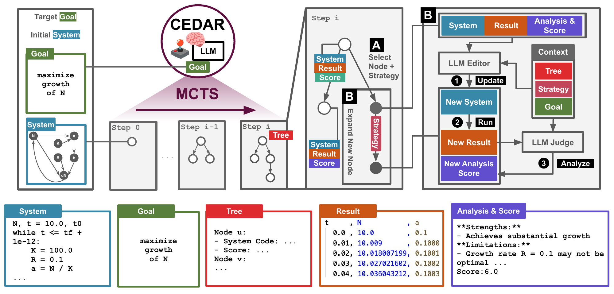
CEDAR architecture: goal and system feed an MCTS loop with LLM Editor and Judge — A goal + an initial system in *restricted Python*. The MCTS tree grows step by step. Each step: **select** a node & strategy, **expand** with the LLM Editor, **run**, **judge**. Each node keeps its system, record, score, and written analysis.

05 / Method: move 1

Represent systems as runnable Python, not a DSL

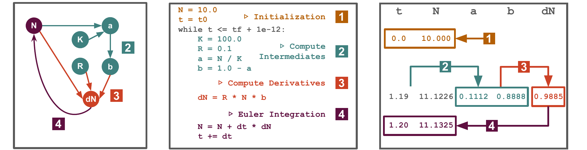
Graph, Python code, and computation table of a population model — Feedback structure as a graph... ...is the same object as plain Python with domain primitives... ...whose run traces every variable at every step.

One representation unifies DYNAMO and STELLA models
Restricted subset + domain primitives + inline docs

LLMs already speak Python fluently
Editing code = editing dynamics: variables, feedback links, equations

Holds all 20 classical systems we study: World Dynamics + 19 from Modeling Dynamic Biological Systems (20–69 integrated variables each).

06 / Method: move 2

LLM Judge as fitness, LLM Editor as variation

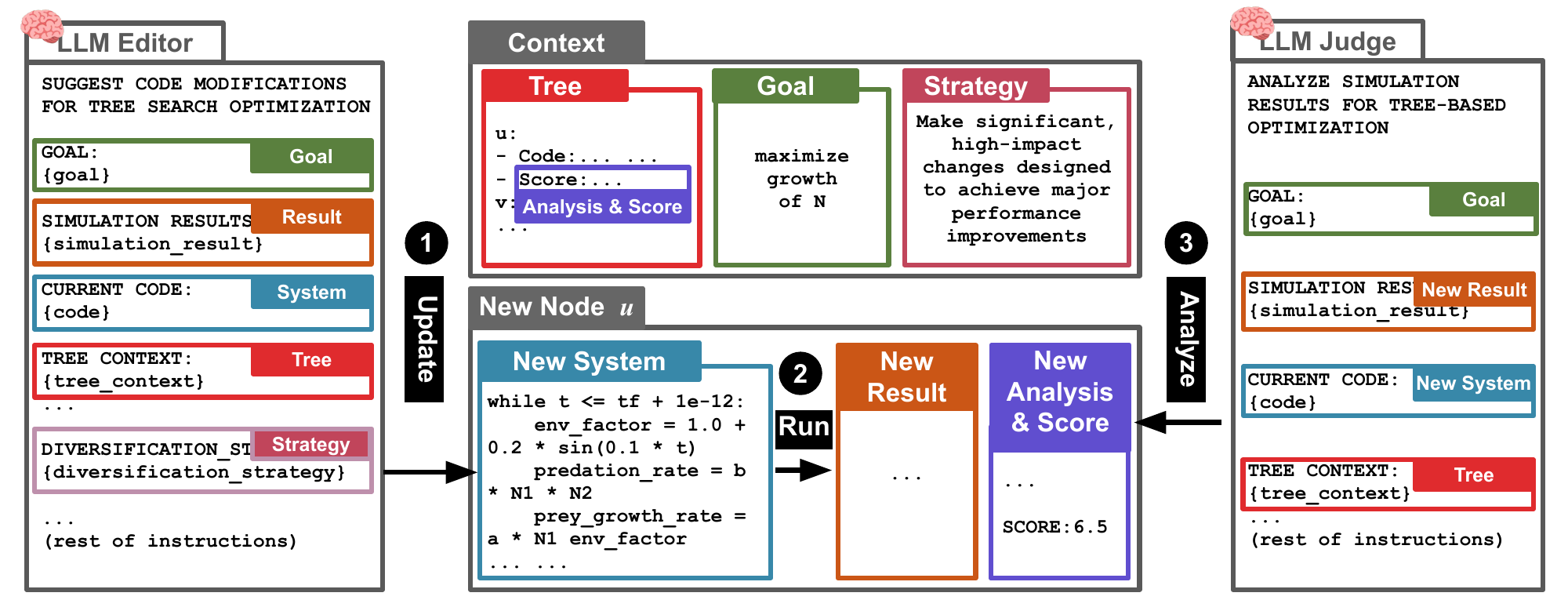
Node expansion: Editor updates the system, it runs, Judge scores and analyzes

Editor (variation operator): structural edits (add/remove state variables, rewire feedback, rewrite equations), guided by strategy, goal, and the parent's analysis.

①→② the Editor writes a new system; running it produces a fresh execution record.

Judge (fitness function): reads the record; returns a bounded score and an analysis that feeds the next edit. A generate-and-evaluate loop, in the spirit of evolutionary computation.

07 / Method: move 3

The search tree is a structured population

Generalized UCT selection

exploration () + depth bonus () + progressive widening ()
nodes re-expandable until , unlike vanilla MCTS
formally a principled MCTS variant: Editor = stochastic transition kernel, Judge = noisy value function

8 expansion strategies, sampled uniformly

breakthrough / aggressive / amplify / exploratory / targeted / contrarian / balanced / conservative

In our runs

backends: Claude Sonnet 4.5 / GPT-5.1
20 selections × 5 candidates
= 100 expansions per search
alpha = 1, gamma = 2

Branching keeps many good, different systems alive at once: selection pressure without collapse. Ablation: MCTS beats linear search (higher scores, smoother search trajectories).

08 / Results: abstract goal

The goal is self-conflicting: pushing one objective breaks the others

World Dynamics already sits near a Pareto frontier
Maximize population only (magenta) ⇒ resources crash, pollution explodes
Minimize depletion only (orange) ⇒ population stagnates

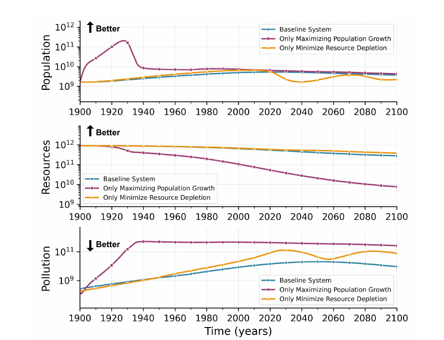
Joint improvement of all three subgoals is the real test.

Single-objective optimization: each subgoal alone damages the others

09 / Results: abstract goal

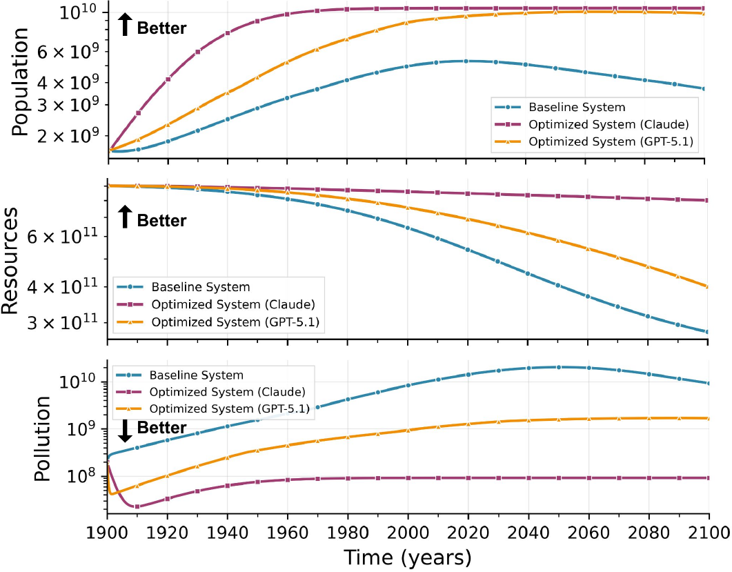
CEDAR finds sustainable worlds: a different one per LLM

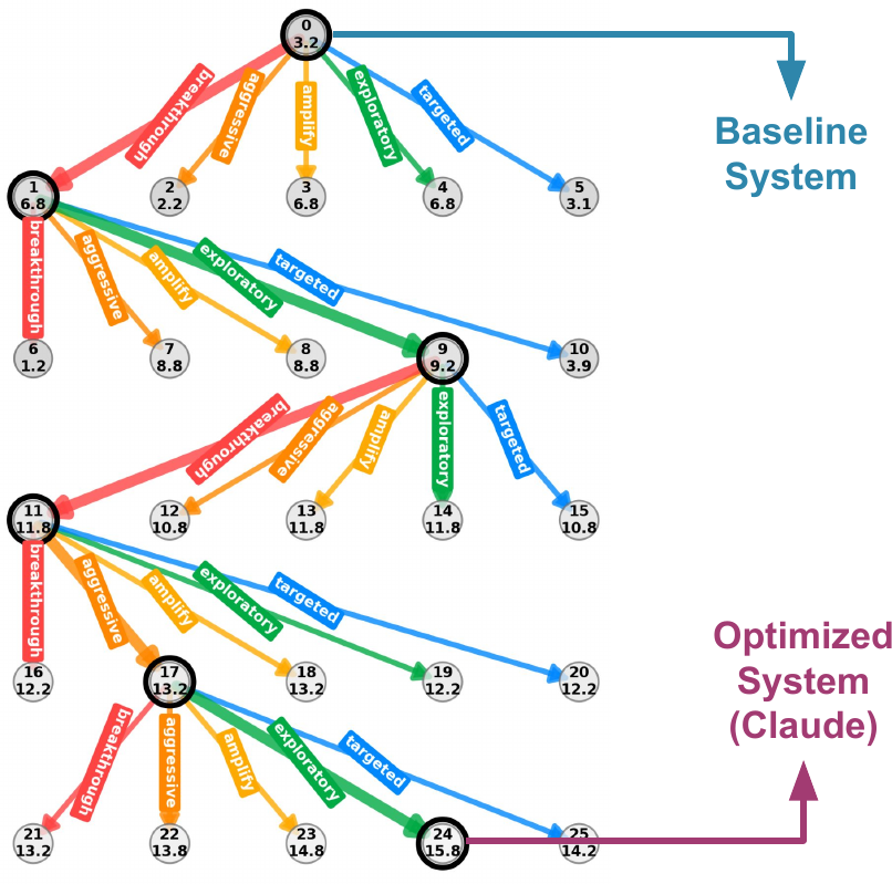
MCTS search tree from baseline to optimized system, best path highlighted

Optimized population, resources, and pollution trajectories versus the baseline system

The tree (left) steers toward higher Judge scores; best path highlighted
Optimized systems (right): population ↑, resources ↑, pollution ↓, all three jointly
Claude and GPT-5.1 discover structurally distinct trade-offs (population-first vs. resource-first)

One vague sentence in, a portfolio of qualitatively different sustainable systems out.

10 / Results: record fitting

CEDAR with no formulae beats Optuna with the full formulae

Task: fit the record of a stochastic population model, starting from a bare skeleton. Optuna gets 100 trials and up to the full ground-truth equations: strictly more prior structure than CEDAR.

Method	Formulae	L1 ↓	DTW ↓
Optuna	none	29.06	5503.68
Optuna	simple	26.01	4927.94
Optuna	full	3.71	477.52
CEDAR (Claude)	none	3.29	757.21
CEDAR (GPT-5.1)	none	2.22	433.13

Without formulae, Optuna collapses to near-constant populations; CEDAR tracks the peaks and dips within ground-truth variability.
Vs. Optuna (full): Claude wins on L1 only; GPT-5.1 wins on both metrics.

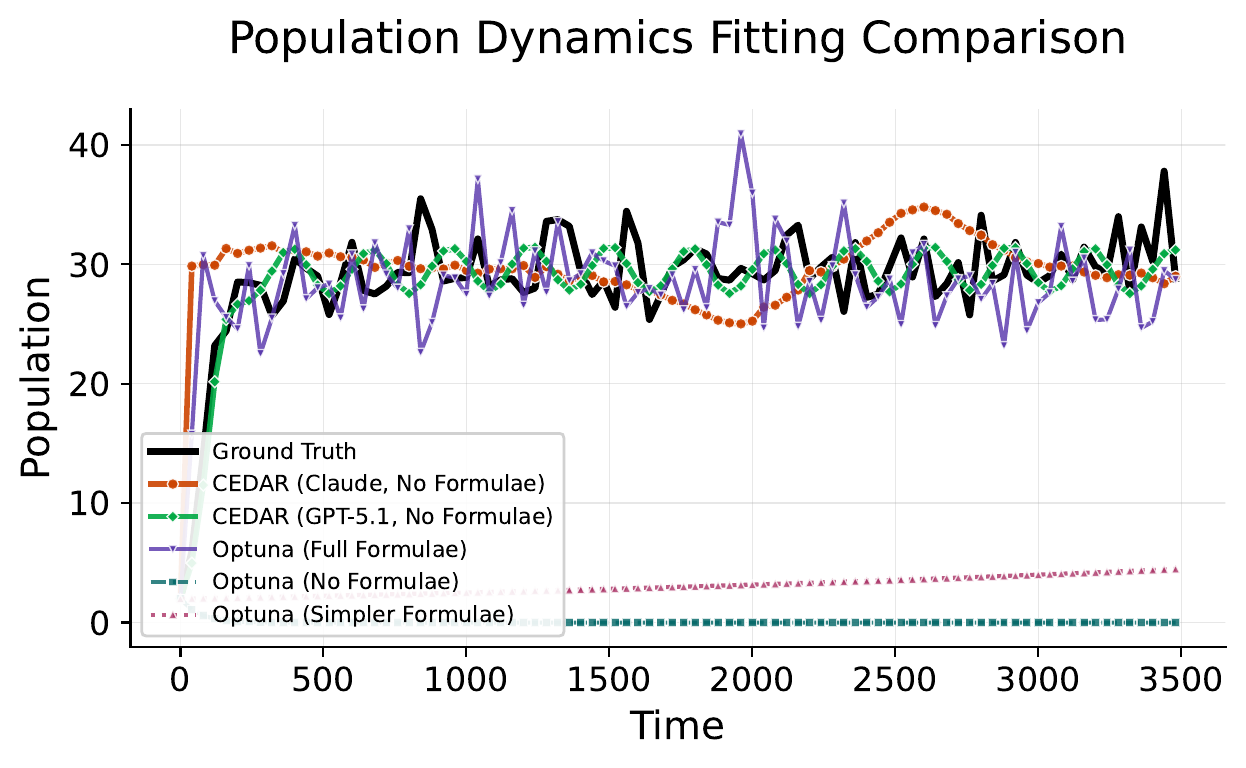
Population trajectories: CEDAR follows ground truth; weak baselines flatline

11 / Results: diversity & interpretability

A population of explained solutions, not a single point

Distinct near-best population trajectories from one run — Near-best nodes of *one* run: all satisfy the goal along *distinct* trajectories ⇒ sensitivity analysis for decision-making.

Every step is narrated.

Judge, at the root: “Unsustainable overshoot behavior - 69% resource depletion, 46x pollution increase”

Judge, at the best node: “Holy grail achievement - 6.4x population growth with only 19.9% resource depletion”

12 / Discussion

For artificial life: range, access, and a record of why

Open-ended exploration. A branching tree preserves structurally distinct emergent behaviors, valuable when the range of behaviors matters, not just one optimum.
Accessibility. Natural-language goals + Python representation lower the barrier that DYNAMO/STELLA workflows impose: complex-systems modeling for more domains, faster decisions.
Transparency. LLM analyses document how structural edits steer emergent behavior, step by step: a new handle on the structure-to-emergence question.

Evolutionary search over living-system models, with agents as its operators.

13 / Method details

One edit cascades across ~45 coupled variables: design needs search

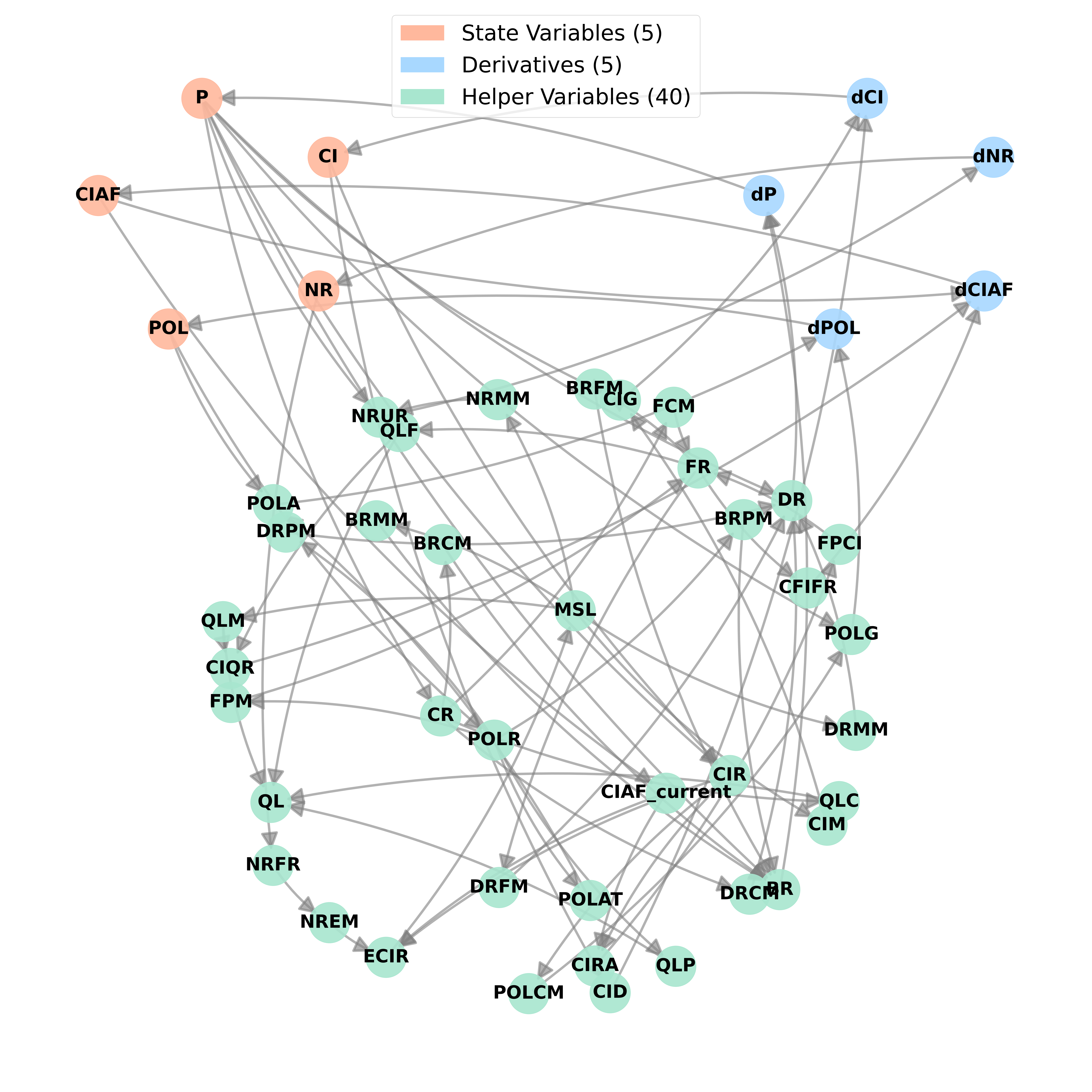
Dependency graph of the World Dynamics system: a dense web of interconnected variables — *World Dynamics* as a dependency graph: ~45 coupled variables; one edit cascades everywhere.

More method details worth mentioning.

enforces progressive widening

Editor: learned transition kernel over programs
Judge: bounded, noisy value function

Engineering for stability

Adaptive context subsampling within budget L; O(NL) total
Structured outputs, up to 3 retries per call
Crashed or NaN runs scored low, so the tree backtracks

14 / Result details

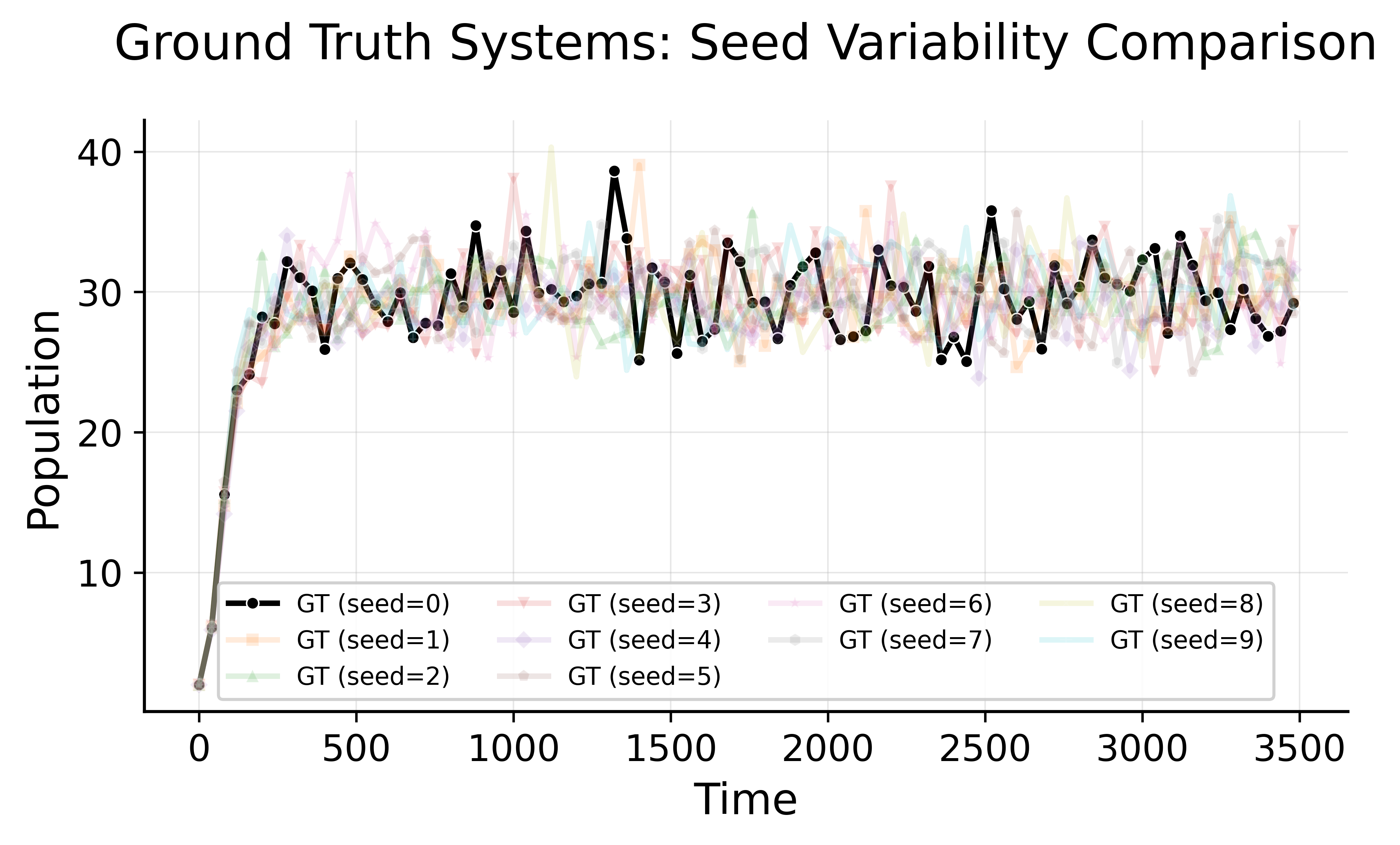
The ground truth is itself volatile: CEDAR fits within the seed band

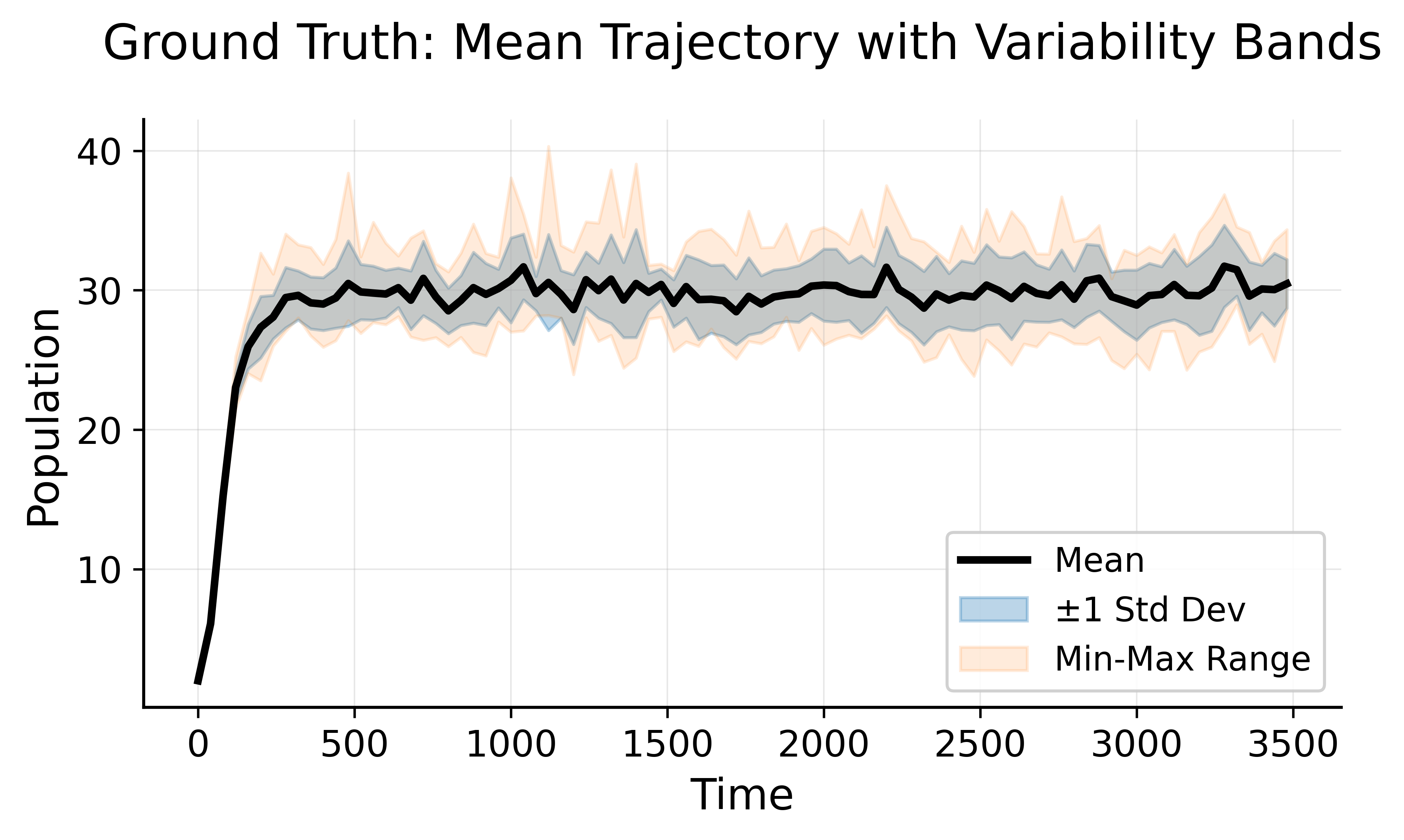
Ground truth trajectories across 10 random seeds with variability band

Overlay of the 10 seed trajectories of the ground truth system

10 random seeds of the ground truth: the stochastic death rate makes the volatility intrinsic, and CEDAR's fit sits within that band.

Method	Formulae	L1 ↓	DTW ↓
Optuna (Run 1)	full	3.71	477.52
Optuna (Run 2)	full	4.26	605.05
CEDAR (GPT-5.1)	none	2.22	433.13

A second full-formulae Optuna run does not close the gap: parameter fitting with the true equations still trails CEDAR (noise floor, sensitive nonlinear landscape).

Full Judge and Editor transcripts are released; scores and reasoning align on human inspection.

15 / Limits & next

Limits, and what comes next

Limits

Judge scores what a same-class LLM edited: circularity risk for abstract goals
Trends, not tight statistics; two systems studied in depth
Judge rationales make the search inspectable, not (yet) a verified causal account of emergence
Convergence guarantees for MCTS-with-LLMs: open

Systematic benchmarks vs. classical evolutionary & multi-objective methods
When is LLM variation/evaluation necessary, not merely helpful?
More systems, more domains

Ask for the behavior.
Let the agents grow the system.

Questions?

Yingtao Tian / Sakana AI / [email protected] / @alanyttian