
How the field builds them: ODEs, Euler, and two old languages

State vector x of meaningful stocks (populations, resources), vector field f, initial values x0 at t0. When f follows a known, simple form, analytical techniques such as the Laplace transform apply.

With nonlinear feedback the field integrates with the first-order Euler method, requiring only that f be computable. Many complex systems admit no analytical solution.
Where the field uses them
Systems thinking that supports policy design and strategic decision-making.
Where f has lived: two old languages
L P.K = P.J + (DT)*(BR.JK - DR.JK)
Outdated syntax or proprietary visual interfaces: both limit their usability with LLMs.
CEDAR in one picture
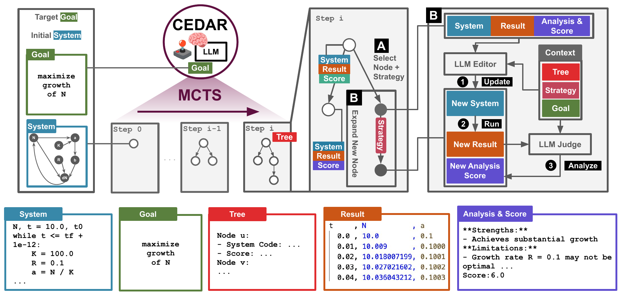
The loop in eight lines: select, expand, run, judge
- 1
 root 0
- 2
 select node to expand
 - 3
 sample expansion strategy
 - 4
 expand
 - 5
 execute
 - 6
 evaluate
 - 7
 add node u; count; drop
 - 8
 track the best; return P*
Symbols, reused from here on
- P the system, a restricted-Python program; G the goal in natural language
- R execution record: values of all variables at each timestamp
- A textual analysis: qualitative feedback and potential improvements
- S bounded numerical score: how well P satisfies G
- cv expansion count of node v;
 its threshold
 - Vexp expandable set: internal nodes stay in it until cv reaches
- Each node keeps

Everything interesting hides in Score, LlmEditor, LlmJudge: the next three moves.
Represent systems as runnable Python, not a DSL
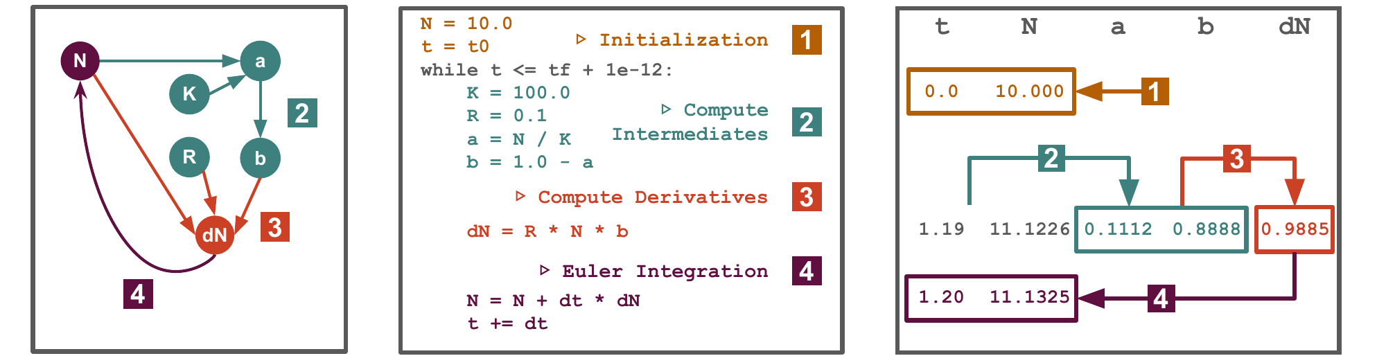
- One representation unifies DYNAMO and STELLA models
- Restricted subset + domain primitives + inline docs
- LLMs already speak Python fluently
- Editing code = editing dynamics: variables, feedback links, equations
Holds all 20 classical systems we study: World Dynamics + 19 from Modeling Dynamic Biological Systems (20 to 69 integrated variables each).
LLM Judge as fitness, LLM Editor as variation
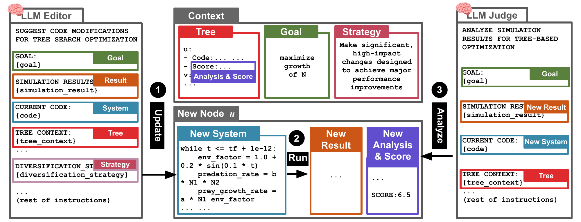
Editor (variation operator): structural edits (add/remove state variables, rewire feedback, rewrite equations), guided by strategy, goal, and the parent's analysis.
①→② the Editor writes a new system; running it produces a fresh execution record.
Judge (fitness function): reads the record; returns a bounded score and an analysis that feeds the next edit. A generate-and-evaluate loop, in the spirit of evolutionary computation.
Scoring: seven bands, two decimals, a depth-limited ceiling
Primary principle: score how well this code achieves the optimization goal, regardless of other nodes in the tree.

Within this limit, high scores are encouraged when performance truly merits them.
Why the tree context is in both prompts
Preliminary studies: without tree context, the expansion process fails to produce meaningful improvements.
The search tree is a structured population
Generalized UCT selection (upper confidence bound applied to trees)
![Score(v) = S_v + alpha * sqrt(ln(c_p+1)/(c_v+1)) * I[c_v < tau] + gamma * Depth(v)](images/f-uct.svg)
- exploration (
 ) + depth bonus (
 ) + progressive widening ()
 - nodes re-expandable until
 , unlike vanilla MCTS
The same loop, in evolutionary vocabulary
| MCTS | Evolutionary computation |
|---|---|
| search tree T | structured candidate population |
| node u with system P_u | candidate system |
| LLM Editor | variation operator |
| LLM Judge | fitness function |
| UCT score, argmax over V_exp | selection |
| re-expand until c_v reaches tau | niche preservation, unlike vanilla MCTS |
Selection is UCT with two twists: progressive widening and a depth bonus
 with
with
![phi = alpha * sqrt(ln(c_p+1)/(c_v+1)) * I[c_v < tau] + beta * I[c_v >= tau] (progressive widening) + gamma * Depth(v) (depth-based bonus)](images/f-phi-braces.svg)
Twist 1: progressive widening
alpha adjusts the amount of exploration; tau controls the expansion count. A node is expandable iff  , and CEDAR sets
  , so a saturated node leaves the race. The cap "prevents overexpansion in vast action spaces like code modification and expensive LLM calls".
Twist 2: depth bonus
gamma > 0 controls the preference for deeper nodes: every extra level adds gamma to the score, so a promising branch keeps being refined.
Why these two, from the appendix
In our runs  , set empirically.
Read formally: the Editor is a transition kernel, the Judge a value function
Eq. 2 / LLM Editor as a learned transition kernel

- a stochastic operator induced by the LLM: a conditional distribution over modified programs
- "extends LLM-powered transition kernels from linear to tree search"
Eq. 3 / LLM Judge as a learned value function

- "Su constitutes a bounded, noisy reward"; semantic LLM scoring is treated as non-adversarial
- "UCT remains consistent when reward noise is bounded and non-adversarial" (Lisy 2013; Efroni 2019)
Twenty classical systems, 100 expansions, about thirty minutes
Data
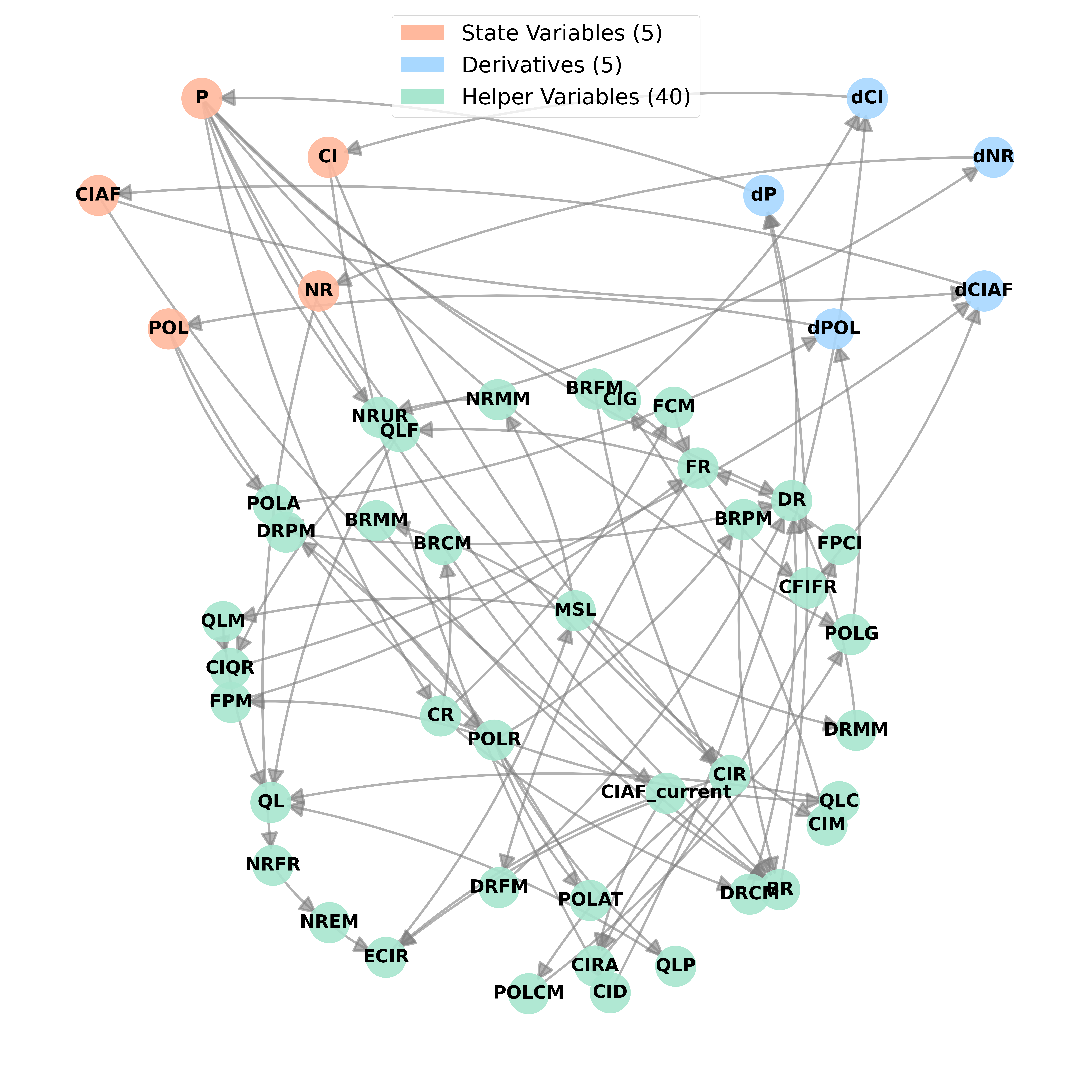
World Dynamics (Forrester 1971) in DYNAMO, plus 19 systems from Modeling Dynamic Biological Systems (Hannon and Ruth) in STELLA, converted into our representation: 20 systems, 20 to 69 integrated variables each.
| Variables | Mean | Max | Range |
|---|---|---|---|
| Integrated | 29.4 | 69 | 20 to 69 |
| Helpers | 10.9 | 12 | 10 to 12 |
Two uses: models to optimize toward goals, and ground truths that produce reference records.
Search
- 20 node selections × 5 new candidates each = 100 expansions per search
- , set empirically
- backends: Claude Sonnet 4.5 and GPT-5.1, default decoding, structured outputs, up to three retries
- crashed or NaN-valued runs get a low score, so MCTS naturally backtracks
Engineering and cost
- each LLM call adaptively subsamples the execution record to stay within a context budget L
- overall
 with N expanded nodes, so large trees and long records scale
 - $10 to $50 per run, about 30 minutes per run
- runtime primarily bounded by LLM calls, not local computation
Experiment 1: one sentence against a web of coupled variables
Why this is hard for World Dynamics, three reasons from the paper:
Cascading effects
With such interdependencies among variables, a single change can trigger cascading effects multiple time steps away.
Competing subgoals
A vague goal decomposes into subgoals that can compete: increasing population typically requires greater resource consumption.
A published Pareto frontier
The baseline is a published system strong enough to sit near a Pareto frontier: pushing one subgoal often comes at the expense of the others.
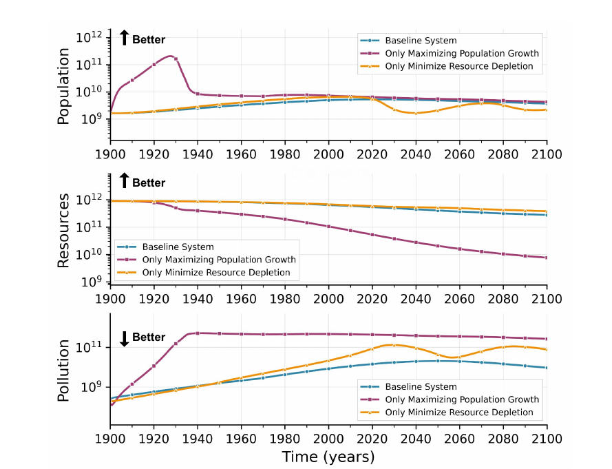
The goal is self-conflicting: pushing one objective breaks the others
- World Dynamics already sits near a Pareto frontier
- Maximize population only (magenta) ⇒ resources crash, pollution explodes
- Minimize depletion only (orange) ⇒ population stagnates
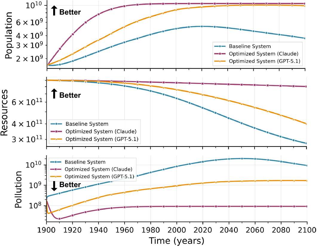
CEDAR finds sustainable worlds: a different one per LLM
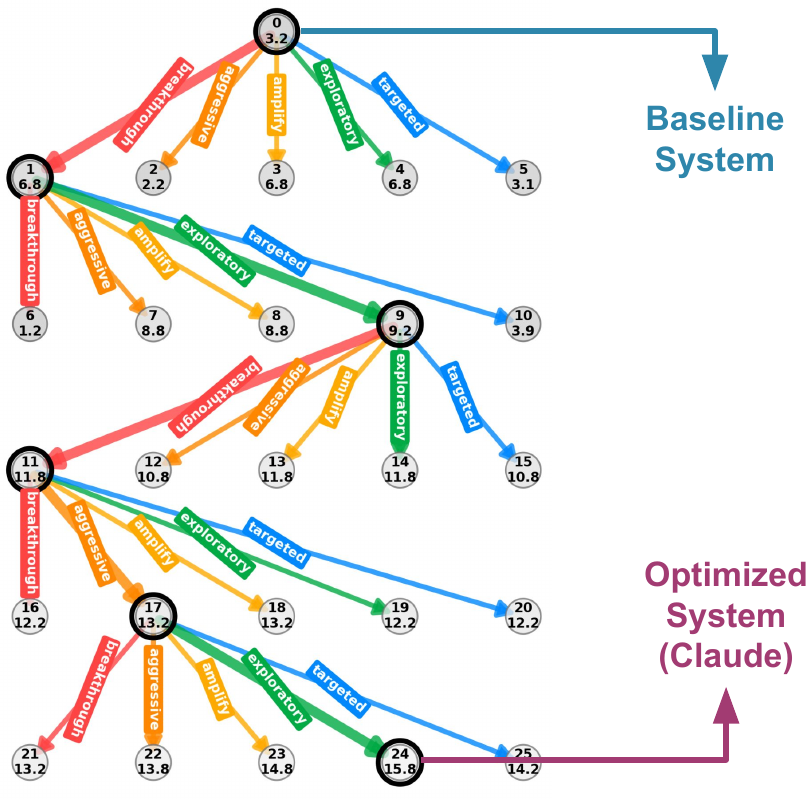
- The tree (left) steers toward higher Judge scores; best path highlighted
- Optimized systems (right): population ↑, resources ↑, pollution ↓, all three jointly
- Claude and GPT-5.1 discover structurally distinct trade-offs (population-first vs. resource-first)
Watch the search climb the tree, one strategy at a time
Editor and Judge responses along the best path, LLM-summarized (Table 3 in the paper)
| node | LLM Editor | LLM Judge |
|---|---|---|
| 0 | (No editor response for root, which is the initial system given as is.) | Unsustainable overshoot behavior - 69% resource depletion, 46x pollution increase |
| 1 | Breakthrough approach - 25-40% efficiency improvements targeting 6-8 score | Sustainable progress - population to 5.46B, 30% resources remaining, controlled pollution |
| 9 | Exploratory approach - radical efficiency through enhanced capital productivity | Paradigm shift - 7.0B population, 78% resource conservation, near-zero pollution |
| 11 | Ultra-aggressive conservation - pushing toward exceptional 9.5+ performance | Breakthrough sustainability - 3.2x population, 36% resource depletion, 90% pollution improvement |
| 17 | Revolutionary breakthrough - 75% resource reduction, 90% pollution control, 300% capital productivity | Best-in-tree performance - 6.3x population, 59% resource conservation, exceptional pollution control |
| 24 | Extreme efficiency breakthrough - 95% resource conservation, 98% pollution reduction, 15x capital productivity | Holy grail achievement - 6.4x population growth with only 19.9% resource depletion |
CEDAR with no formulae beats Optuna with the full formulae
Task: fit the record of a stochastic population model, starting from a bare skeleton. Optuna gets 100 trials and up to the full ground-truth equations: strictly more prior structure than CEDAR.
| Method | Formulae | L1 ↓ | DTW ↓ |
|---|---|---|---|
| Optuna | none | 29.06 | 5503.68 |
| Optuna | simple | 26.01 | 4927.94 |
| Optuna | full | 3.71 | 477.52 |
| CEDAR (Claude) | none | 3.29 | 757.21 |
| CEDAR (GPT-5.1) | none | 2.22 | 433.13 |
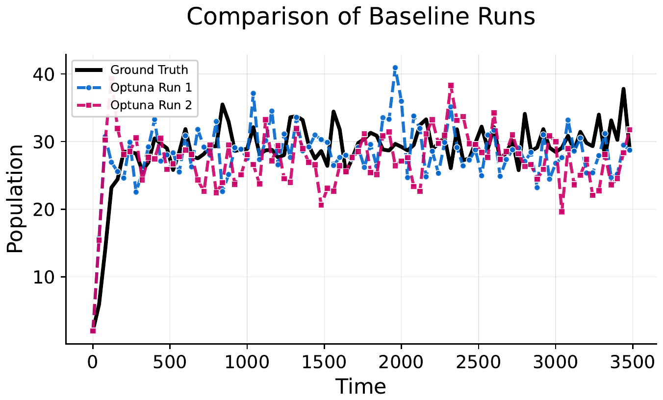
Without formulae, Optuna collapses to near-constant populations; CEDAR tracks the peaks and dips within ground-truth variability.
Vs. Optuna (full): Claude wins on L1 only; GPT-5.1 wins on both metrics.
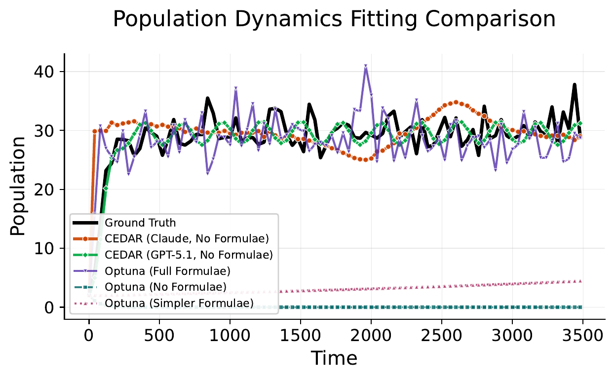
The ground truth is itself volatile: CEDAR fits within the seed band
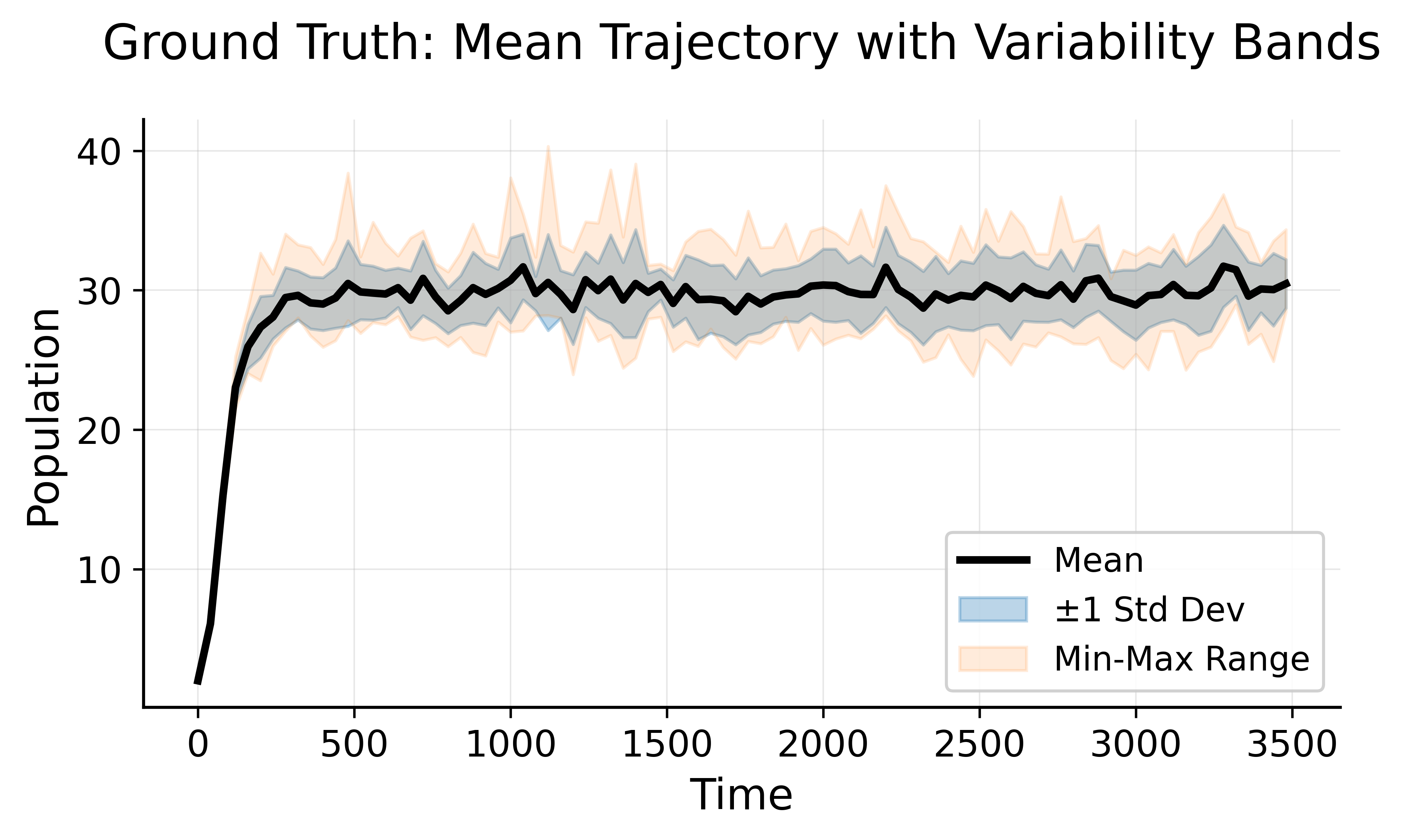
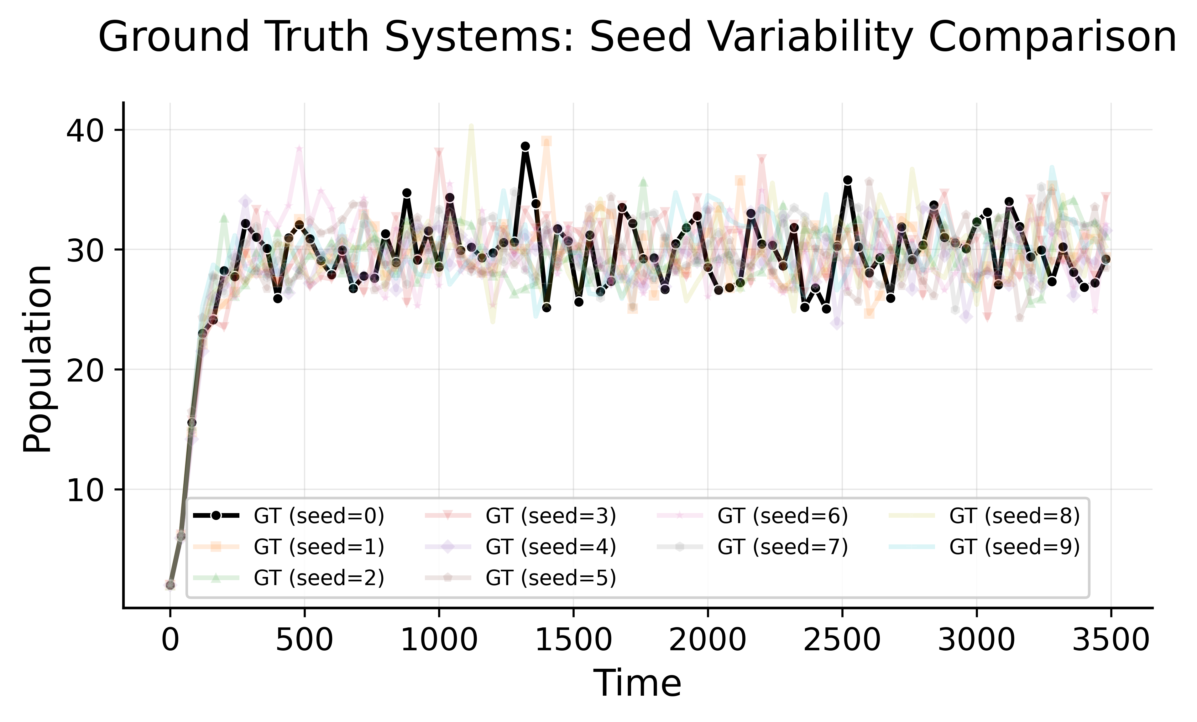
10 random seeds of the ground truth: the stochastic death rate makes the volatility intrinsic; CEDAR's record (previous slide) generally falls within this band.
DR_DISTRIBUTION = normal(NOMINAL_DR, 0.005 * POPULATION)
The death rate is sampled at every time step from a normal distribution parameterized by the current population, so peaks and dips are not in sync across runs: the volatility is an intrinsic property of the system, not an artifact of the optimizer.
A second full-formulae run does not close the gap: why parameter fitting trails
| Method | Formulae | L1 ↓ | DTW ↓ |
|---|---|---|---|
| Optuna (Run 1) | full | 3.71 | 477.52 |
| Optuna (Run 2) | full | 4.26 | 605.05 |
| CEDAR (GPT-5.1) | none | 2.22 | 433.13 |
In theory, with full formulae access and enough trials, Optuna could approach the ground truth system's parameters. In practice it does not perfectly match the dynamics. Two factors:
- The noise floor. Visible in the ground truth itself: peaks and dips are not in sync across runs.
- A hard landscape for purely numeric search. The parameter space is high-dimensional and sensitive: "small changes can lead to qualitatively different records" through nonlinear feedbacks.
Near-best nodes of one run: a population, not a point

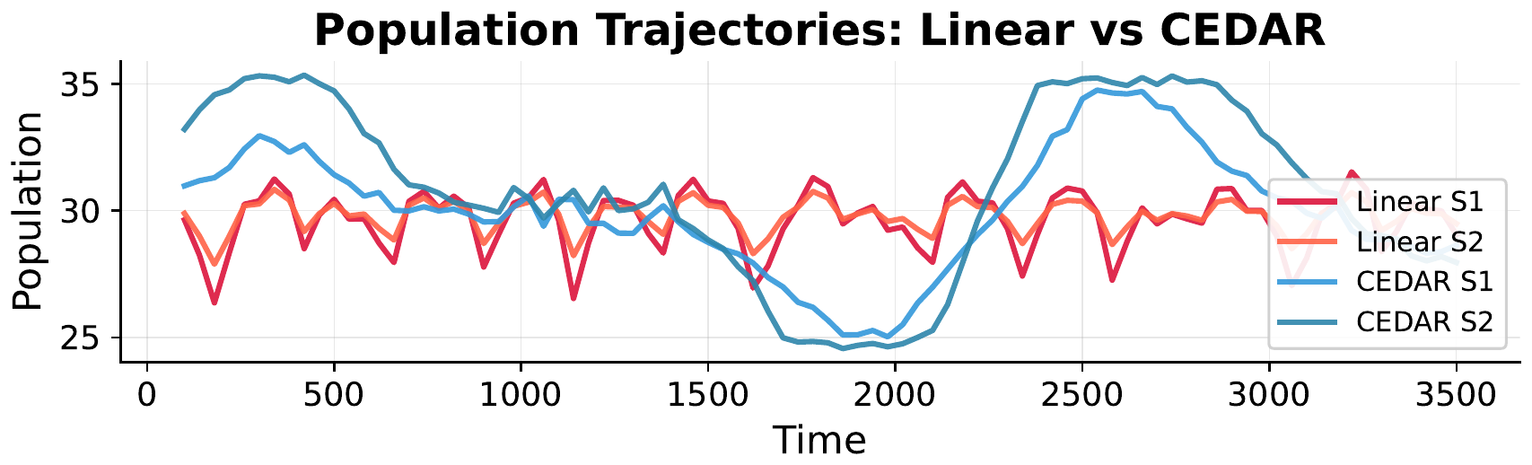
- Diversity. Nodes within a single run whose scores are close to the best all satisfy the goal, yet follow distinct trajectories; unlike the Optuna baselines, CEDAR avoids collapsing to a single overfitting-like point, which enables better decision-making through sensitivity analysis.
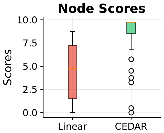
- Performance. MCTS yields higher-scoring nodes than linear search (next slide).
- Open-ended discovery. A branching tree, rather than convergence to a single point, preserves structurally distinct high-performing systems, each emphasizing different trade-offs among objectives.
Ablation: the tree beats the line, in score and in dynamics
Let the agents grow the system.
Questions?
Yingtao Tian / Sakana AI / [email protected] / @alanyttian